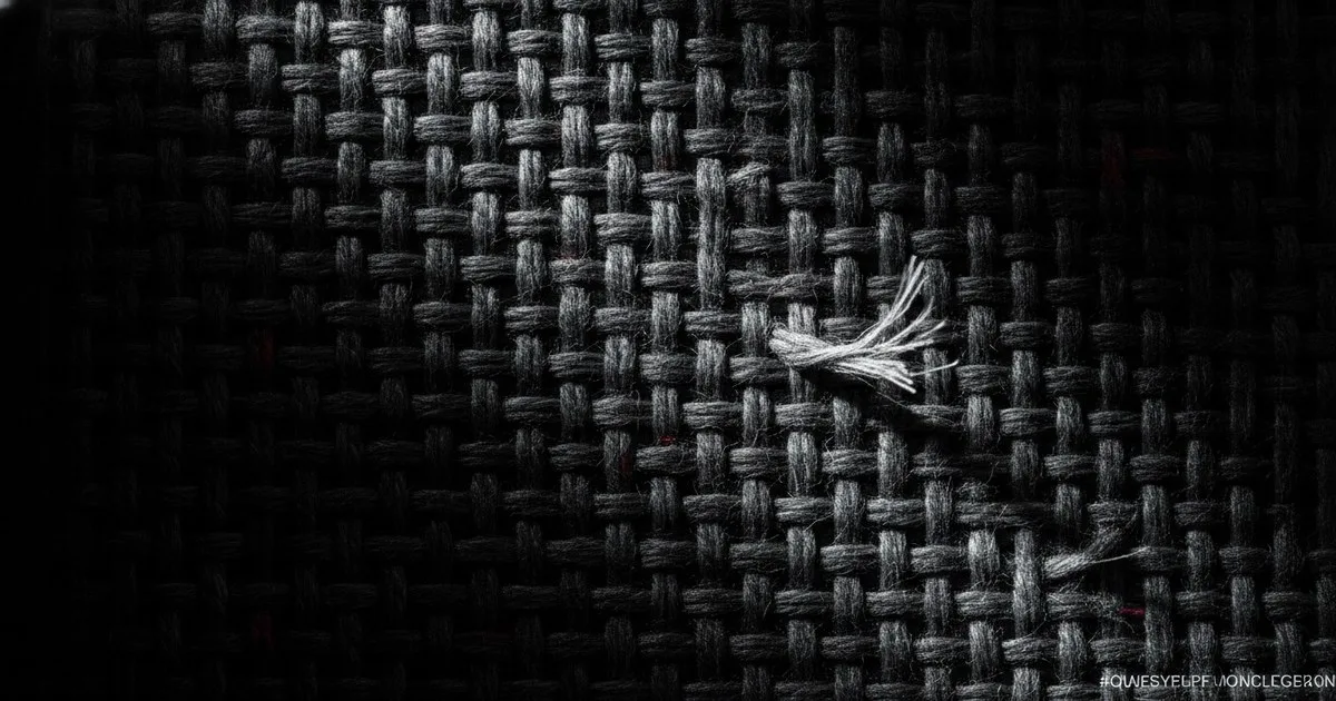
A model inspecting woven fabric does not see a defect. It sees a near-periodic texture and a local violation of that periodicity; the class name, the severity grade and the accept-or-reject decision are bolted on afterwards. That reframing decides your architecture, because modelling normal weave is a different problem from classifying faults you have almost no examples of.
Key takeaways
- Woven fabric is a stationary, near-periodic texture, so the real modelling target is what normal looks like, not what each defect looks like.
- Backbones pretrained on natural photographs carry object priors with no analogue in fabric, and the resizing they assume destroys the yarn-level detail defects live in.
- Class imbalance is structural rather than fixable: a healthy production line emits almost no defective samples.
- Pixel-accurate masks and a stable defect dictionary are the scarce resources, not model capacity or GPU hours.
- Illumination geometry and camera choice move final accuracy more than swapping one architecture for another.
What does a textile defect actually look like to a model?
Acquisition constrains everything downstream. Inline inspection usually means a line-scan camera over moving fabric under fixed illumination, producing a continuous strip rather than discrete photographs. Resolution is set by the smallest fault you must catch, often the scale of a single yarn.
Defects then divide by what they perturb:
- Geometry of the weave. Missing or doubled yarns, floats, misdraws, holes and thin places break the repeat, appearing as phase and frequency anomalies. This class suits periodicity modelling best.
- Local mass. Slubs, knots and neps add material without breaking the repeat, reading as intensity blobs whose signature depends on the lighting angle.
- Colour and shade. Stains, barré and shade bands are wide-area, low-frequency deviations. A patch classifier cannot see them, because a small crop holds no reference for the correct shade.
- Surface finish. Crease marks, pilling and abrasion are texture-statistic changes rather than discrete objects, and graders disagree about them more than any other class.
No single receptive field covers all of that: yarn-level faults need fine detail, shade bands need wide context. Illumination is part of the model too. A hole is obvious in transmitted light and nearly invisible in diffuse reflection; surface relief is the reverse. Choose an architecture before fixing the optics and you spend the project compensating for something a lamp would have solved.
Which architectures are used, and what does each assume?
| Approach | What it assumes | Where it breaks |
|---|---|---|
| Patch classifier on a convolutional backbone | A defect is decidable from a local crop | Blind to wide-area shade and barré; needs labelled patches per class |
| Fully convolutional segmentation | You can supply pixel masks | Thin linear faults make annotation slow and annotators inconsistent |
| Reconstruction anomaly detection | Trained only on good fabric, the residual reveals the fault | A capable decoder learns to reconstruct the defect too |
| Feature-memory comparison against normal patches | Mid-level features of normal fabric cluster tightly | Sensitive to changeover; the memory bank must be rebuilt per construction |
| Vision transformer with windowed attention | Long-range attention captures repeat structure and shading | Data-hungry; patch tokenisation can straddle the weave repeat and blur phase |
| Frequency-domain preprocessing feeding any of the above | The weave is genuinely periodic | Knits, jacquards and irregular constructions violate the assumption |
The useful systems are hybrids. A frequency or Gabor-style front end suppresses the regular weave so the residual carries the anomaly; a convolutional or attention model then classifies what survived. Reconstruction and feature-memory methods cover fault types nobody labelled, which matters because a mill will meet faults absent from your taxonomy.
Why does transfer learning from ImageNet underperform on woven fabric?
Because the pretraining task rewards exactly the invariances you need to destroy.
Object priors do not transfer. Early layers learn edges, gradients and colour opponency, which are genuinely reusable. Later layers learn object parts and their arrangement, and fabric has no parts and no layout, so much of the pretrained representation is dead weight you pay to fine-tune.
Scale and shape of the input. Natural-image backbones expect a subject filling much of a square frame, and standard augmentation assumes the same. A defect occupies a tiny fraction of a long strip: resize and the yarn-level evidence is interpolated away, tile instead and you inherit crops with no wide-area context.
Invariance in the wrong direction. Pooling and strided convolution deliberately discard precise position. Detecting a missing pick is a phase measurement against a periodic reference, exactly the information those layers throw out.
What works better is unglamorous: pretrain with a self-supervised objective on the unlabelled good fabric your line already produces, keep the early layers, retrain from mid-level upward, train at native resolution, and put shade assessment in a separate wide-context model.
What is the labelling bottleneck, and how do you work around it?
Masks for thin faults are slow to draw and inconsistent between annotators, so boundary disagreement caps any pixel-level metric. Taxonomies are unstable, because mills name faults differently and categories overlap. Imbalance is structural: a line running well produces almost nothing to learn from. Labels are noisy too, since the same roll graded twice does not always get the same verdict.
The workarounds that hold up:
- Train on normal fabric only and treat detection as anomaly scoring, so you stop depending on defect volume.
- Use the weak labels you already have: a manual inspection log gives roll-level verdicts, enough to supervise a coarse model and to prioritise annotation.
- Inject synthetic faults into real good-fabric images — yarn removal, local warping, stain compositing — accepting that the model learns your generator, and generator artefacts become shortcuts.
- Run active learning against the residual, annotating only frames the current model finds ambiguous.
- Maintain a versioned defect dictionary with reference crops per class, and recompute historical metrics when it changes. This is the step that gets skipped, and the one that quietly invalidates a year of measurements.
Where do material scanning and 3D pipelines connect to this?
The same controlled-capture discipline shows up on the design side. Vizoo builds the xTex hardware and software system for high-resolution physically based material scanning, plus a platform for acquiring physical fabric properties, used in 3D apparel workflows. A scanning rig is the inspection problem in reverse: fixed geometry, repeatable lighting, calibrated colour, because everything downstream inherits whatever error capture introduced.
Those measured properties then drive simulation. Browzwear ships a 3D product creation platform — VStitcher, Lotta and SmartDesign — using physics-based simulation, AI-assisted fit validation and connections into product data systems to cut physical sampling. Fidelity there depends on measured material behaviour rather than nicer rendering, the same lesson inspection teams learn about optics.
NVIDIA Research, the research organisation of NVIDIA Corporation, publishes across generative AI, rendering and robotics and releases open-source code libraries. Rendering research matters here because a renderer that reproduces real illumination response is the difference between synthetic training data that transfers and synthetic data that teaches shortcuts.
Related reading here: our walkthrough of how diffusion models generate fashion images covers texture synthesis from the generative side, and the argument for treating garment geometry as model input explains why raster imagery alone loses structure a pattern keeps.
What is still unsolved?
Open-set recognition and grading. Production reliably produces faults absent from your taxonomy, and accept-or-reject thresholds differ per customer. Anomaly scoring finds the fault; naming and grading it still needs a human, so the work shifts rather than disappears.
Domain shift and evaluation. A model tuned on one loom, fibre blend and colour range degrades on the next, and continual adaptation without catastrophic forgetting is still open. Public texture-anomaly datasets are cleaner and better lit than any mill, so scores on them say little about line performance.
FAQ
Is a convolutional network or a transformer better for fabric inspection? Neither dominates. Convolutional models are stronger on fine local faults at limited data volumes; attention models handle wide-area shading and long repeats. Most systems pair a frequency-based front end with one of them.
Can I train a defect detector without labelled defects? Yes. Reconstruction and feature-memory methods train on good fabric only and score anomalies by deviation from normal. You still need labels to name and grade faults, but detection no longer waits on collecting rare positives.
Why does my accuracy collapse when the fabric changes? Because the model learned one construction's texture statistics. Changeover alters weave density, sheen and colour, shifting the feature distribution. Rebuild the normal reference per construction, and evaluate per fabric family rather than reporting one aggregate score.
What should I fix before touching the model? Optics and logging. Get illumination geometry, resolution and exposure stable, then record every frame with machine, batch and operator verdict attached. Both cost less than architecture work and explain more of the outcome.
Further reading
- Applications of Computer Vision in Fashion and Textiles — an edited volume covering textile defect detection and quality control alongside recognition and body modelling.
- Fashion Meets Computer Vision: A Survey — a survey of how detection underpins most downstream fashion vision tasks.
- Computer Vision for Fashion: A Systematic Review — a review of where computer vision has been applied across fashion design and production.